Discriminative model

There are many ways to classify machine learning algorithms: supervised/unsupervised, regression/classification,… . For myself, I prefer to distinguish between Discriminative model and Generative model. In this article, I will discuss the relationship between these 2 families, using Gaussian Discriminant Analysis and Logistic Regression as example.

Quick review: Discriminative methods model $p(y \mid x)$ . In classification task, these models search a hyperplane (a decision boundary) seperating different classes. The majority of popular algorithms belongs to this family: logistic regression, svm, neural net, … On the other hand, Generative methods model $p(x \mid y)$ (and $p(y)$ ). This means that it will give us a probability distribution for each class in the classification problem. This give us an idea of how the data is generated. This type of model relies heavily on Bayes rule to update the prior and derive the posterior. Some well-known examples are Naive Bayes, Gaussian Discriminant Analysis, …

discriminative_vs_generative — Discriminative vs Generative. Source: evolvingai.org.

There are quite some reasons why discriminative models are more popular among machine learning practitioner: they are more flexible, more robust and less sensitive to incorrect modeling assumptions. Generative models, on the other hand, require us to define the distribution of our prior, which can be quite challenging for many situations. However, this is also their advantage: they have more “information” about the data than discriminative model, and thus can perform quite well with limited data if the assumption is correct.

In this article, I will demonstrate the point above by proving that Gaussian Discriminant Analysis (GDA) will eventually lead to Logistic Regression, and thus Logistic Regression is more “general”.

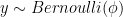
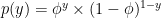
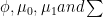
For binary classification, GDA assumes that the prior follows a Bernoulli distribution and the likelihood follows a multivariate Gaussian distribution:

$y \sim Bernoulli(\phi)$

$x \mid y=0 \sim N(\mu_0, \sum)$

$x \mid y=1 \sim N(\mu_1, \sum)$

Let’s write down their mathematical formula:

$p(y) = \phi^{y} \times (1-\phi)^{1-y}$

$p(x \mid y=0) = \frac{1}{(2\pi)^{n/2} |\sum|^{1/2} } \times exp(- \frac{(x - \mu_0)^T(x - \mu_0)}{2 \sum })$

$p(x \mid y=1) = \frac{1}{(2\pi)^{n/2} |\sum|^{1/2} } \times exp(- \frac{(x - \mu_1)^T(x - \mu_1)}{2 \sum })$

As mentioned above, the discriminative model (here is the logistic regression) try to find $p(y \mid x)$ , so what we try to prove is that:

$p(y=1 \mid x) = \frac{1}{1 + exp(-\theta^T x)}$

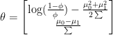
which is the sigmoid function of logistic regression, where $\theta$ is some function of of $\phi, \mu_0, \mu_1 and \sum$ .

Ok let’s roll up our sleeves and do some maths:

$p(y=1 \mid x)$

$=\frac{p(x \mid y=1) \times p(y=1)}{p(x)}$

$= \frac{p(x \mid y=1) \times p(y=1)}{p(x \mid y=1) \times p(y=1) +p(x \mid y=0) \times p(y=0)}$

$= \frac{1}{1 + \frac{p(x \mid y=0) \times p(y=0)}{p(x \mid y=1) \times p(y=1)}}$

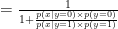
This equation seems very much like what we are look for, let’s take a closer look at the fraction $\frac{p(x \mid y=0) \times p(y=0)}{p(x \mid y=1) \times p(y=1)}$ :

$\frac{p(x \mid y=0) \times p(y=0)}{p(x \mid y=1) \times p(y=1)}$

$= exp(-\frac{(x - \mu_0)^2}{2 \sum} + \frac{(x-\mu_1)^2}{2 \sum} ) \times \frac{1 - \phi}{\phi}$

$= exp(\frac{(x-\mu_1)^2 - (x-\mu_0)^2}{2 \sum}) \times exp(\log(\frac{1-\phi}{\phi}))$

$= exp(\frac{(\mu_0 - \mu_1)(2x-\mu_0-\mu_1)}{2\sum}) \times exp(\log(\frac{1-\phi}{\phi}))$

$= exp(\frac{2(\mu_0 - \mu_1)x - (\mu_0 - \mu_1)(\mu_0 + \mu_1)}{2 \sum} +\log(\frac{1-\phi}{\phi}))$

$= exp(\log(\frac{1-\phi}{\phi}) - \frac{\mu_0^2 + \mu_1^2}{2\sum} + \frac{\mu_0 - \mu_1}{\sum} \times x )$

$= exp[ (\log(\frac{1-\phi}{\phi}) - \frac{\mu_0^2 + \mu_1^2}{2\sum}) \times x_0 + \frac{\mu_0 - \mu_1}{\sum} \times x ]$

In the last equation, we add $x_0 = 1$ so that we can have the desired form $\theta^Tx$ . The former equation is then:

$\frac{1}{1 + \frac{p(x \mid y=0) \times p(y=0)}{p(x \mid y=1) \times p(y=1)}} = \frac{1}{1 +exp[ (\log(\frac{1-\phi}{\phi}) - \frac{\mu_0^2 + \mu_1^2}{2\sum}) \times x_0 + \frac{\mu_0 - \mu_1}{\sum} \times x ] }$

And there it is, we just proved that the result of a Gaussian Discriminant Analysis is indeed a Logistic Regression, our vector $\theta$ is:

$\theta = \begin{bmatrix}\log(\frac{1-\phi}{\phi}) - \frac{\mu_0^2 + \mu_1^2}{2\sum} \\ \frac{\mu_0 - \mu_1}{\sum} \end{bmatrix}$

The converse, is not true though: $p(y \mid x)$ being a logistic function does not imply $p(x \mid y)$ is mutlivariate gaussian. This observation shows us that GDA has a much stronger assumption than Logistic Regression. In fact, we can go 1 step further and prove that if $p(x \mid y)$ belongs to any member of the Exponential Family (Gaussian, Poisson, …), its posterior is a logistc regression. We see now a reason why Logistic Regression is widely used: it is a very general, robust algorithm that works for many underlying assumptions. GDA (and Generative models in general), in the other hand, makes much stronger assumption, and thus is not ideal for non-Gaussian or some-crazy-undefined-distribution data .

(The problem of GDA, or generative model, can be solved with a class of Bayesian Machine Learning that uses Markov Chain Monte Carlo to sample data from their posterior distribution. This is a very exciting method that I’m really into, so I will save it for a future post.)